The Shape of a Calculation: A Geometric View of Arithmetic: Part 1

In the world of AI, the famous analogy “king – man + woman = queen” reveals a hidden geometric structure in our language. This inspired a bold question: Does simple, everyday arithmetic also have its own unique “shape”? What if we treated basic operations like “+1” and “×2” not as mere instructions, but as movements across an uncharted map? But as we began to draw this map, we discovered something startling…

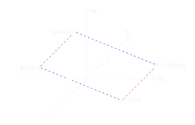
Our story begins, as many modern tales of structure and meaning do, with the famous word embedding analogy:

king – man + woman = queen

This equation is captivating because it suggests that meaning is not arbitrary. It has a shape. In the world of word embeddings, concepts like “king” and “woman” are represented as points in a high-dimensional space. The relationships between them, like “gender” or “royalty,” are represented as vectors—the directed lines connecting these points. The magic of the parallelogram is that the vector from “man” to “king” is nearly identical to the vector from 1 “woman” to “queen.” This observed geometric regularity is what allows us to navigate the space of meaning.

But the standard approach has a subtle hierarchy: the concepts (words) are primary entities (points), while the relationships (vectors) are secondary, derived from the positions of the points. The regularity is a beautiful, but often approximate, emergent property.

This led us to a different, more radical question. What if we take this regularity not as a mere observation, but as a strict, foundational law? What if we build a world where the relationships themselves are just as fundamental as the concepts they connect? In such a world, an operation like “add one” wouldn’t just be something you do to a number; it would be a first-class geometric entity, on equal footing with the number itself. This single philosophical shift—treating concepts and relations as peers—is the true starting point of our journey. It forces us to ask: what kind of geometry emerges when we demand this perfect, universal regularity?

The First Test: The Analogy Breaks

The most basic place to test this new principle is arithmetic. Our concepts are numbers (like an arbitrary number α), and our relations are operations (like “+1” and “×2”). If we demand universal regularity, then the order in which we apply these relations shouldn’t matter for the geometry. A parallelogram should form.

Let’s run the experiment. We have two paths from α:

1.Path 1 (Apply relation “+1”, then “×2”): (α + 1) × 2 = 2α + 2
2.Path 2 (Apply relation “×2”, then “+1”): (α × 2) + 1 = 2α + 1

Immediately, our strict principle leads to a contradiction. The two paths don’t lead to the same result. The parallelogram fails to close.

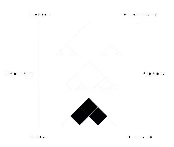
This isn’t just a failed analogy anymore. It’s the first major discovery yielded by our new principle. It tells us that a geometry where concepts and relations are peers cannot be the simple, flat Euclidean space we’re used to. The operations of addition and multiplication are not commutative, and this non-commutativity must be a fundamental feature of our new geometric world.

The Complexity Explosion and the Need for a New Geometry

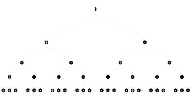
This failure has a staggering consequence. Since the order of operations matters, every unique sequence of operations creates a distinct arithmetic expression. (α + 1) × 2 is fundamentally different from (α × 2) + 1 . This leads to a combinatorial explosion. The number of possible expressions grows exponentially with the number of operations. Think of it as a vast, ever-branching “library of all possible calculations.”

Now, imagine that each of these unique expressions must occupy a unique region in our geometric space. How much “room” would we need? In a standard Euclidean space (the flat space of high school geometry), the volume of a ball grows polynomially with its radius (e.g., r² for a circle, r³ for a sphere). A space with polynomial growth is like a small bookshelf; it simply cannot contain an exponentially growing library. It would run out of room almost immediately.

This forces us to look for a different kind of geometry, one whose capacity grows exponentially. The math itself is telling us that our familiar, flat world is not the right stage for this play. Fortunately, such a geometry exists: hyperbolic space. The failure of the parallelogram is not a bug; it’s a feature pointing us directly toward a curved, hyperbolic world.

A Quick Tour of Hyperbolic Space

So, what is this “hyperbolic space”? The easiest way to understand it is to start with the “flat” Euclidean space we all know. A defining rule of flat space is the parallel postulate: through a point not on a line, there is exactly one line parallel to the given line. Hyperbolic geometry is what happens when you change this rule.

In hyperbolic space, through a point not on a line, there are infinitely many lines parallel to the given line.

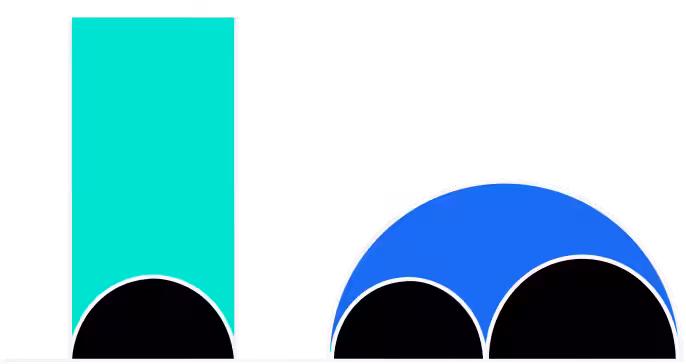
It’s hard to picture this in your head, but a good analogy is the surface of a saddle or a Pringles chip. This shape has what’s called “negative curvature.” On such a surface, lines that you might think are parallel actually curve away from each other, opening up more and more space between them.

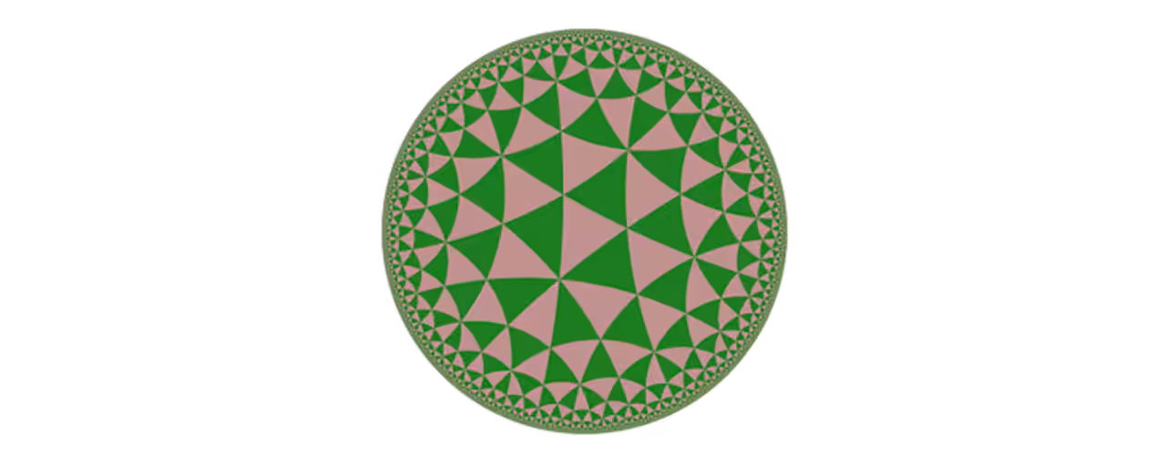
This “curving away” has a dramatic effect: the space expands much faster than flat space. As mentioned, the area or volume of a circle in this space grows exponentially with its radius. This boundless, rapidly expanding nature is precisely what we need. It provides more than enough “room” to house the exponential complexity of arithmetic expressions. A visual way to feel this is through the famous “Circle Limit” woodcuts by M.C. Escher, which are artistic renderings of hyperbolic space. Notice how the angels and demons appear to shrink as they get closer to the edge, allowing an infinite number of them to fit within a finite circle.

Drawing Hyperbolic Space: The Upper Half-Plane Model

The saddle and Escher analogies are helpful for intuition, but to do real work, we need a concrete map. One of the most powerful ways to draw hyperbolic space is the upper half-plane model.

Imagine the standard 2D plane with coordinates (x, y) . The upper half-plane is simply the entire region where y > 0 . The magic lies in how we define “distance” and “straight lines” (geodesics) on this map.

• Distance is deceptive: The geometry is distorted. The deeper you are in the plane (the smaller y is), the “smaller” your ruler becomes. As you move up toward larger y values, your ruler effectively “grows,” and you can cover what appears to be a large distance with very few steps. The x-axis at y=0 is a boundary that is infinitely far away from any point within the plane. A journey from y=1 to y=0.1 is vastly longer than a journey from y=10 to y=9 .
• Straight lines are curved: A “straight line” is the shortest path between two points. In this distorted map, the shortest paths take two forms: This might seem strange, but this model perfectly captures all the rules of hyperbolic geometry. Most importantly for us, it gives us a concrete coordinate system (x, y) to build our theory upon.

With this new kind of space in mind, we can now return to our quest.

A New Physics for Numbers: The Flow Equation

Instead of thinking of numbers as static points, what if we imagine their evaluation as a dynamic process? Let’s build a thought experiment. Imagine a tiny boat on a strange sea. This sea has two forces acting on the boat:

1. A constant current that always pushes it in one direction (say, “north”). This is our additive force.
2. A strange “stretching” of the water itself, which pushes the boat “east” with a force that depends on how far from the “southern shore” it already is. This is our multiplicative force.

What path will the boat trace? The mathematical description of this path is what we call the Flow Equation: = ds da μ cos θ + aλ sin θ

Let’s break down this equation, connecting it back to our boat analogy:

• da/ds : This is the velocity of our value, a , as we move a tiny distance ds through our geometric space.
• μ cosθ : This is the additive drive. It’s the constant current. The parameter μ is its strength. This term represents addition.
• aλ sinθ : This is the multiplicative drive. It’s the “stretching” force, proportional to the current value a . The parameter λ is its strength. This term represents multiplication.
• θ : This is simply the direction the boat is steering. If it steers purely “north” (θ=0), it only feels the additive current. If it steers purely “east” (θ=90°), it only feels the multiplicative stretching. Steering at any other angle mixes the two forces.

The parameters μ and λ are like the “arithmetic genes” of the space, defining its fundamental character. This equation suggests that we can build a geometric space where movement itself encodes arithmetic. But does such a space actually exist?

The answer is yes. And the first concrete, “miraculous” example is a mathematical object we call the first kind arithmetic expression space (E1). We can build it on the very map we just discussed: the hyperbolic upper half-plane.
On this space, we can draw a grid where movement along the horizontal blue lines corresponds to addition, and movement along the vertical green lines corresponds to multiplication. Moving left or right changes the x coordinate, which adds or subtracts from our value. Moving up or down changes the y coordinate, which scales (multiplies or divides) our value.

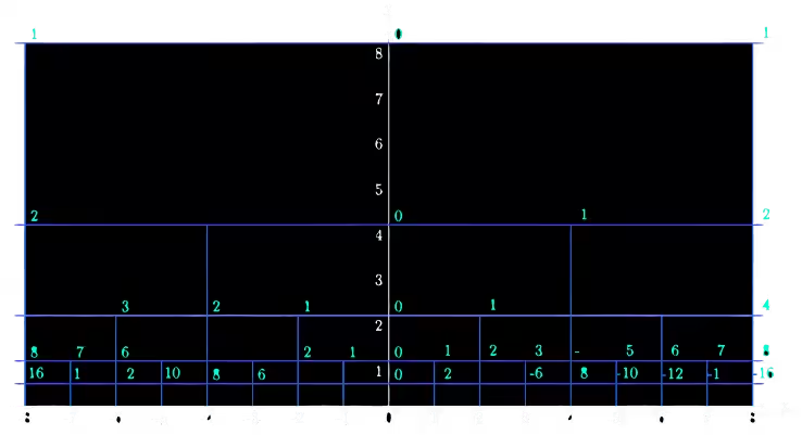
After all this abstract reasoning, the most remarkable part is that there exists an elegant, almost shockingly simple function that assigns a value to every point (x, y) on this grid: a=−x/y

This space, with this grid and this assignment function, is a perfect solution to our Flow Equation. The abstract idea of a “flow” suddenly becomes a concrete, visualizable reality. We have found a geometry that naturally embodies the rules of arithmetic.

Paths as Calculations: A Visual Demonstration

Now that we have this geometric stage—the E1 space—let’s see it in action. This grid isn’t just a static map; it’s a visual calculator. Every path you can draw on it corresponds to a specific arithmetic expression.

Let’s trace the expression (1 × 8) – 5. The goal is to start at a point with value 1 and arrive at a point with value 3.

1. Start at 1: We find a point on the grid where a = -x/y = 1 . One such point is (x=-8, y=8).
2. Multiply by 8: Multiplication changes the scale, which corresponds to moving vertically along a green line. To multiply our value by 8, we must divide our y coordinate by 8. We move from (x=-8, y=8) straight down to (x=-8, y=1) . Let’s check the value here: a = -(-8)/1 = 8. Perfect.
3. Subtract 5: Addition/subtraction corresponds to moving horizontally along a blue line. To subtract 5 from our current value of 8, we must add 5 to our x coordinate (because of the negative sign in a = -x/y ). We move from (x=-8, y=1) to the right to (x=-3, y=1) . The final value is a = -(-3)/1 = 3 .

The path, shown in black in the diagram below, is a simple L-shape.

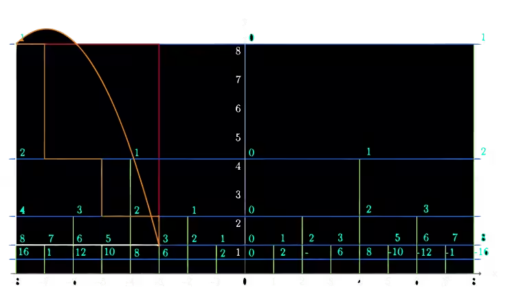
But this isn’t the only way to get from 1 to 3. Consider the algebraically equivalent expression (1 – 5/8) × 8 . This traces a completely different path (shown in purple):

1. Start at 1: We begin again at (x=-8, y=8).
2. Subtract 5/8: First, we perform the subtraction. To subtract 5/8, we add 5/8 to x. But wait, our y coordinate is 8. The formula a = -x/y means a horizontal step’s value depends on its y level. To subtract a value of 5/8 at y=8, we need to change x by (5/8) * 8 = 5. We move from (x=-8, y=8) to (x=-3, y=8). The value here is a = -(-3)/8 = 3/8.
3. Multiply by 8: Now, we multiply by 8. We move vertically down from (x=-3, y=8) to (x=-3, y=1). The final value is a = -(-3)/1 = 3.

We have found two distinct geometric paths that are algebraically equivalent. They start at the same point and end at the same point. This raises a fascinating question: What is the deep geometric principle that governs this equivalence? What is the meaning of the area between these paths?

This is the mystery we will unravel in Part 2.

At Sapient Intelligence, we believe that true innovation often comes from revisiting the most fundamental questions with a fresh perspective. We encourage our researchers to embark on ambitious, long-term explorations, even into territories that seem familiar. The theory we had shared, the Geometry of Arithmetic Expressions, is the result of such a journey—one that has spanned nearly a decade. It began with a simple, almost naive question, and has since blossomed into a new way of seeing the very structure of calculation.